Semantle + Connections Write Up

Semantle, Connections, and word relationships

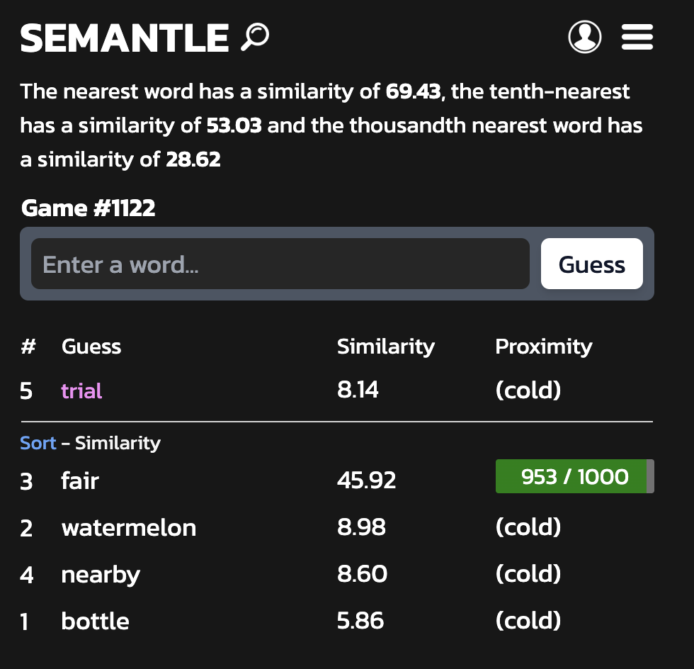
Semantle is a game where you try to guess the secret word based on the “similarity” of the other words you guessed

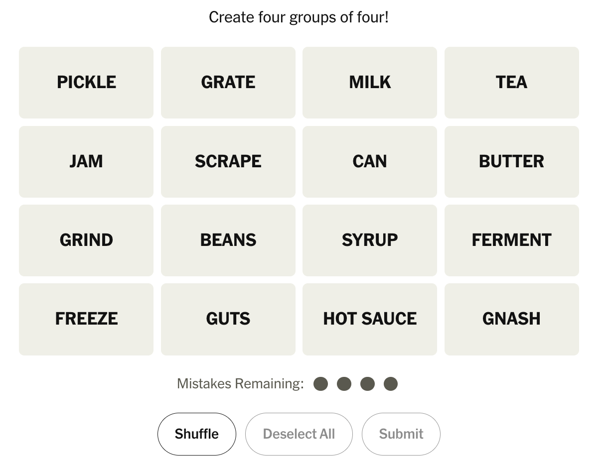
[NYT Connections](https://www.nytimes.com/games/connections
(https://www.nytimes.com/games/connections) is a game where you sort words into groups of four based on similarity or patterns.

… So, what do these two games have in common?
They both deal with the relationships between words! Semantle is relatively straightforward, with the player just trying to find one unknown word with the context of the previous guesses. Connections requires players to think about four potential categories simultaneously and sort the words based on their relations.

How to quantify word relationships: Word2Vec

Thinking about how to solve these as humans is pretty straightforward. While individual people’s understandings of the world will naturally differ, we (at least those of us who would log in and play these games) have shared context and with a little trial and error we can come to the same conclusions.

How can we quantify words?
We can represent word relationships as vectors in high dimensional space. This allows us to capture both semantic and syntactic relationships between words, in turn letting us analyze these relationships mathematically.

Word2vec is a popular method in natural language processing (NLP) for obtaining vector representations of words.

1. It uses a shallow, two-layer neural network to process text and produce a high-dimensional vector space (usually between 100 and 300 dimensions)
   • It’s trained on large text corpora to learn the context of the words
2. Then, each unique word in the corpus is assigned a corresponding vector in the space
   • The model adjusts weights to reduce a loss function (measures how well the model’s predictions match the actual target values)
   • The hidden layer weights becoming the word embeddings
3. Words with similar meanings or contexts are positioned closer together in the vector space, thus capturing semnatic meaning

What did we use?
We used a dataset callsed “googlenews-vectors-negative300”
It’s pre-trained on Google News with 3 million words in 300 dimensions.
2 main models: CBOW and Skip-gram
We used CBOW, which stands for Continuous Bag of Words.
It’s a neural network-based algorithm that predicts a target word given its surrounding context words.

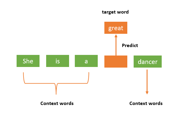
Architecture of CBOW

1. Input Layer: A fixed-size window of context words surrounding a target word (in the above example, 4 context words). Each word is typically represented as a one-hot encoded vector.
   A one-hot encoded vector is a binary vector used to represent categorical data in a format that can be processed by machine learning algorithms.
   It is a $1\times N$ matrix where $N$ is the number of categories in the data.
   Each category is represented by a unique vector with all zeros except for a single one at the index corresponding to that category.
   For example, these would be the one-hot vectors of “She is a great dancer"
   "She”: $\left[\begin{array}{ccccc}1& 0& 0& 0& 0\end{array}\right]$
   “is”: $\left[\begin{array}{ccccc}0& 1& 0& 0& 0\end{array}\right]$
   “a”: $\left[\begin{array}{ccccc}0& 0& 1& 0& 0\end{array}\right]$
   “great”: $\left[\begin{array}{ccccc}0& 0& 0& 1& 0\end{array}\right]$
   “dancer”: $\left[\begin{array}{ccccc}0& 0& 0& 0& 1\end{array}\right]$
   Note that the order of these is arbitrary, and N is equal to the number of unique words in the corpus.
   To train a word, the one-hot vectors of the words inside the context window are summed into a single training vector.
   If the window size is 3 before and 1 after (like in the picture), the training context vector for “great” would be $\left[\begin{array}{ccccc}1& 1& 1& 1& 1\end{array}\right]$ (sum of all the relevant one-hot vectors)
2. Embedding Layer: This layer maps the one-hot encoded input vectors to their corresponding dense vector representations or embeddings.
   • transforms high-dimensional categorical data into lower-dimensional, dense vector representations.
3. Average: The model computes the average of the context word embeddings to create a single vector representing the combined context.
4. Hidden Layer: The averaged embedding vector is passed through a hidden layer, which performs a non-linear transformation using an activation function like tanh or ReLU.
5. Output Layer: The output layer is a linear layer that maps the hidden layer’s output to the target word embedding.

Skip-gram

1. Input and Output:
   • Takes a target word as input and tries to predict its surrounding context words
2. Training Process:
   • generating paris of (target word, context word).
   • The model uses these pairs to maximize the probability of predicting context words given the target word.
3. Neural Network Architecture:
   • The skip-gram model typically consists of an input layer (the target word), a hidden layer (where embeddings are learned), and an output layer (representing the context words).
   • During training, the weights are adjusted to minimize prediction errors

The Differences
CBOW: predicts a target word based on its surrounding context words.

• takes multiple context words as input and aims to estimate the probability of the target word occurring in that context
  Skip-gram: Predicts the surrounding context words based on a single target word.

• uses the target word to predict multiple context words
  CBOW is generally faster, making it more ideal for larger datasets. Skip-gram is better for smaller datasets or when it’s important to represent rare words effectively.

We can use math to analyze relationships between words:
cosine similarity - Measures the angle between two vectors, ranging from -1 to 1.

• $cos(90)=0$, meaning that lines at a right angle are the most dissimilar
• $\cos (\theta )=\frac{A\cdot B}{\Vert A\Vert \Vert B\Vert }$ - A dot B divided by their magnitudes
  dot product - similar to cosine similarity but also accounts for magnitudes of the vector
• $A\cdot B=\Vert A\Vert \Vert B\Vert \cos (\theta )$
  euclidean distance - the length of the line segment between two points in Euclidean space
• Euclidean distance gets less effective in higher dimensions
  the “curse of dimensionality”: the relative contrast between the nearest and farthest points to diminish as dimensionality increases
  things get pushed to the edges of n-space, leaving the center empty
  the relative distances between points become less meaningful
  • i.e. looking at only the x coordinate on a number line vs in 3D space
• Basically Pythagorean theorem in $R^{300}$
  vector addition - adding vectors of equal dimensions, taking into account both magnitude and direction (which in this case represent semantic meaning)
• for example, “King” - “Man” + “Woman” = a vector near to “Queen”
  Clustering - a technique used to group similar entities based on their content, meaning, or style
• an unsupervised machine learning method
• used to discover patterns, themes, or relationships within large collections of text data
• common algorithms include K-means, hierarchal clustering, and DBSCAN

Solving Proximity

Proximity is a game similar to Semantle, where you try to guess a secret word. Instead of giving us the distance between our guess and the target word like Semantle does, Proximity gives us how close we are to the word (based on semantic similarity). For example, if a guess is “5 away,” it means there are only 4 words in the entire dataset that are semantically closer to the secret word than the guess.

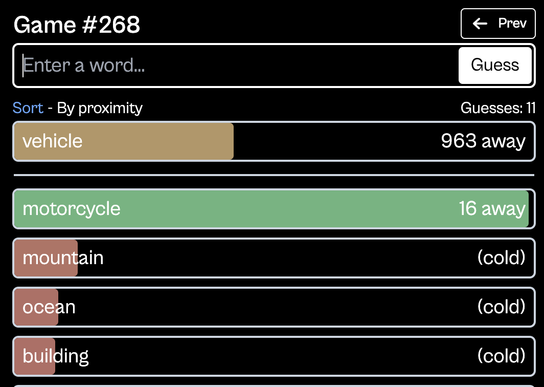
*Proximity starts giving you the distance once you are within the 100 closest words

Here’s how we tried to solve it:

Instead of taking a similarity score, we took the distance the word was from the target. Then, we found the $x$ most similar words to our guess.
This… didn’t work.

To solve it, we would need to compare the rankings of this word in relation to every other word in the database. In the example above, this would look like:

1. iterating through the dataset

2. for each word, rank the top 16 most similar words

3. repeat until you find a word that has ‘motorcycle’ as the 16th most similar word
   This would be very intensive computationally, to say the least - ($O(n^2)$)
   there’s probably ways to simplify this, but anything already takes ages to run on my computer, so we decided it’s best not to

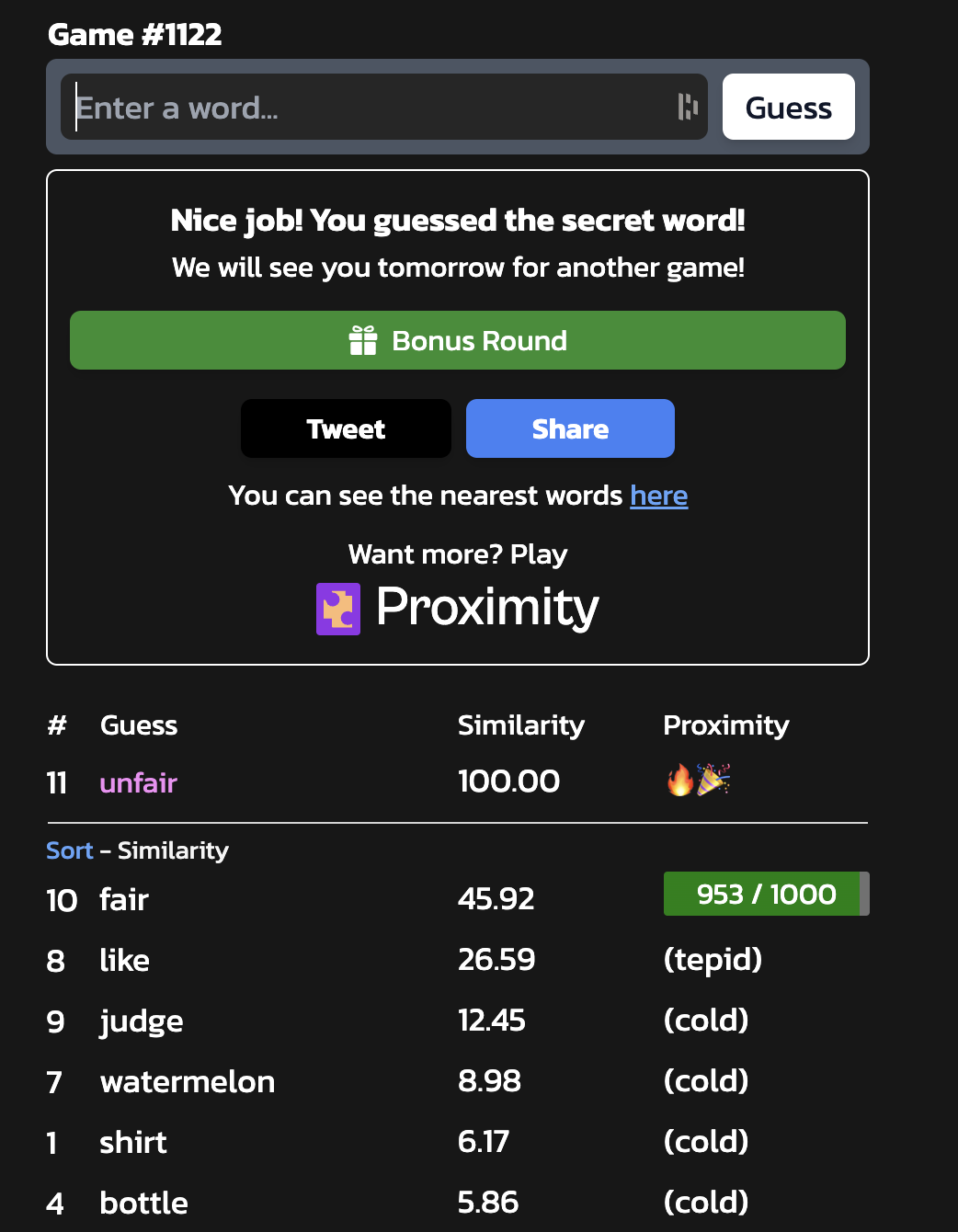
Solving Semantle

When we enter a guess, Semantle gives us feedback in the form of a “similarity score,” which tells us the cosine distance ($1-\text{cosine similarity}$) between the vector for our guess and the secret word.

Since we have the dataset that the game used (GoogleNews-vectors-negative300), we can use the feedback given to find the word.
We take two guesses and their similarity scores as input. Then, for each word that is $x$ distance away from the first guess, we check if it is also $y$ distance away from the second guess.
Finally, we remove any words with underscores ”_” because they are not in the solution set for Semantle.
This results in the answer to the puzzle.

We used the library Gensim, a popular open-source Python library for natural language processing (NLP). It’s primary focus is on unsupervised topic modeling and semantic vector representation of documents. 
Gensim processes raw, unstructured text data using unsupervised machine learning algorithms. It represents words/documents as semantic vectors, capturing the underlying meaning and relationships between them.

KeyedVectors is a model in Gensim that stores and manages word vectors or word embeddings. It’s essentially a mapping between entities (usually words) and their corresponding vector representations in a high-dimensional space.

1080 possible connections…

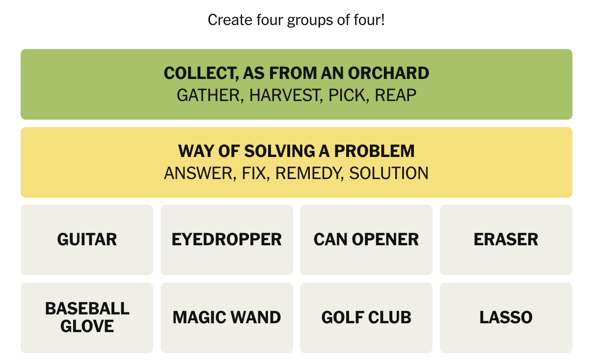
Unlike Semantle, connections is written by a human. Wyna Liu sits down and thinks with her mushy human brain to come up with the categories. This means that while Proximity and Semantle can be solved by using the same calculations and dataset that they use internally, solving connections relys on the word2vec dataset as an NLP tool, not just a lookup table.

The New York Times Connections game board has 16 words that we’re supposed to group into four categories.
There are 16c4 possible ways to do this: a 1 in 1080 chance to get it right with pure luck (0.0926% chance!).

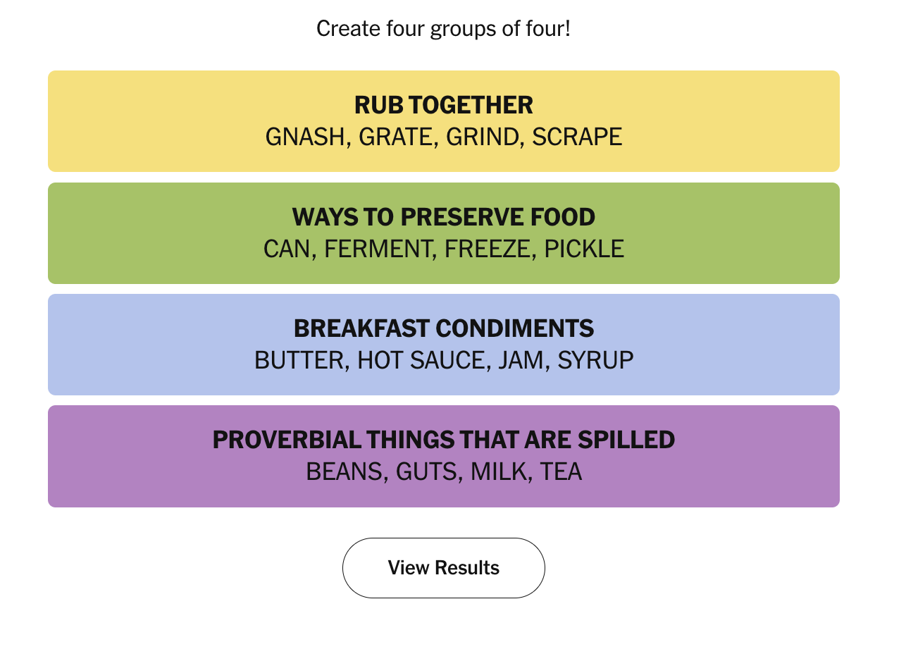
There are a few types of categories (non-exhaustive list):

• items in a set based on literal meaning (i.e. office furniture)
• examples of things (i.e. ways to preserve food)
• items in a set, not based on meaning (i.e. football teams)
• word-play (i.e. palindromes, ends in a number)
• ___ word or “words that come after ___“
  The less concrete categories tend to be the harder ones for us to guess (blues, purples)
  We predicted that these would be not be as similar semantically / not as close in the word2vec model and thus would be harder for our algorithm to guess.

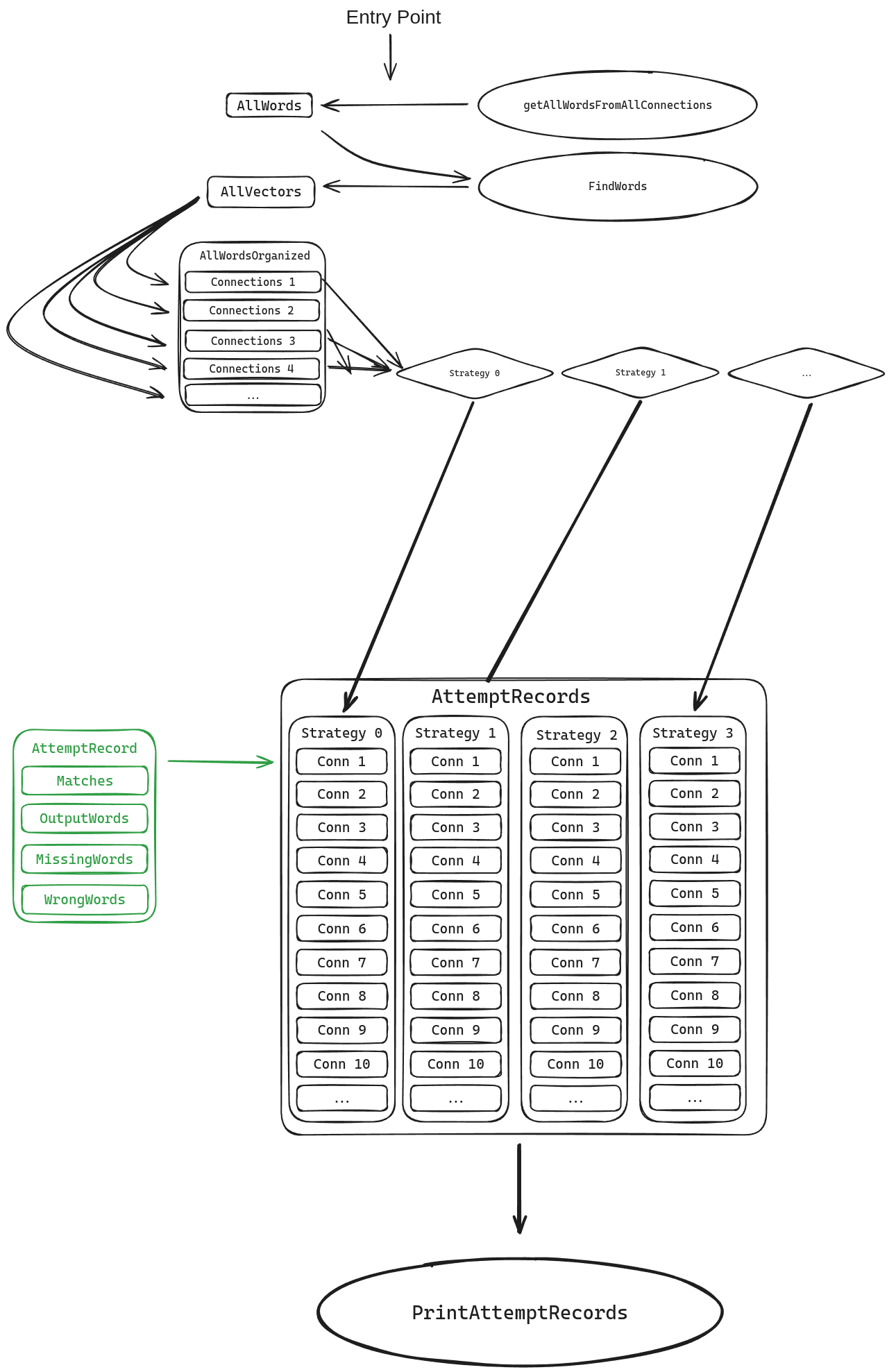
How does the program work?

Embeddings Capture

We wrote a simple python script to print all the embeddings in the google news model we downloaded into a simple text file. This file ended up being well over 13 GB. An AWK script processes the fairly dirty output export into single line entries with space delimitation, which is much easier to handle in C.

Our laptops have 15 GB of ram, and while we could technically parse and load the entire set into memory, it would be tight, and unnecessary. Instead, a retrieval function takes a list of words and iterates through the embeddings file line by line, only parsing and storing the embeddings of desired words. It’s pretty important that all the words for all the subsequent operations are captured in one shot, rather than capturing the 16 or 4 words of interest in smaller chunks, because of the 12 second execution time, about 10 seconds are spent searching through the embeddings.

Because we searched the file for all the words at once, they end up in a one level list, but they need to be organized into a map (AKA dictionary) whose keys are the identifier numbers of each connections game. I wrote this conversion really naively, and I expect it to break easily, but it works right now.

Processing Structure & Output Capturing (Analytics)

Each strategy (described later) is assigned a number. I tried to setup the processing structure so a single function could be handed the 16 words for a connection and the strategy number, and then it would just deal with it. This didn’t really work, so I wasn’t able to put all the attempts in a loop. Instead, there’s 4 blocks that look almost identical in the main function, each starting the processing for a particular strategy.

Each strategy takes the 16 words and 16 embeddings for them, and then tries to pick out 4 words that go together which are returned in an icky way that we never standardized.

Those 4 blocks each have a loop which increments through the map of words and vectors, passing all 16 words and their vectors into the right strategy function. That function returns “something that never got standardized”, which is entered by some ugly code into a storage structure called attemptRecords. It’s split by strategy, then by connection game, and contains the number of words it got right (matches), the list of words it returned, a list of words it returned but that weren’t right, and a list of words that were right, but it didn’t return. The category it’s return is compared against is calculated seperately and is just the first category in the connection that has the most matching words as the return.

After the program runs, there’s some code to output the output storage structure as readable text in the terminal and as a .csv file for graphing and stuff.

Strategies

We wrote 4 algorithms to pick out 4 similar words from 16 words. They are as follows

	Euclidean Distance	$\frac{1}{\text{dot product}}$ Distance
Brute Force	0	1
K-Means	2	3

Brute Force:
The brute force function generates a map (dictionary) where the keys are $R^4$ vectors of integers, where the integers are the indicies representing both a word and it’s embedding vector. The value associated with each key is the calculated average distance between each of those 4 words and their centroid. The distance can be either Euclidean (strategy 0) or cosine/$\frac{1}{dot}$ distance (strategy 1)

K-Means Clustering:
It starts by specifying the number of clusters ($K$) you want to create. Each cluster is represented by a centroid, which is the mean of all points in that cluster. The centroid is picked randomly at the start. Then, Each data point is assigned to the cluster whose centroid is closest to it (usually by Euclidean Distance).
After all points are assigned, the centroids are updated to be the mean of all points assigned to each cluster. This is repeated until the centroids don’t change significantly.

The final results might not be what we expected. When I made this randomly, I expected the clusters to be 1-8-2, 3-4-7, and 5 and 6 kinda being off to the side. Maybe 6 would have joined 1, 8, and 2. To be fair, this is a really simple example, and I only ran the algorithm once.
This goes to show that the locations of the initial centroids have an impact on the final clusters. Take a look at this example with a different initial centroids:

The final groups are 1-8-2, 3-4-7, and 5-6—different from the first time.

Euclidean Distance:
Used in strategies 0 and 2, takes two vectors and returns the square root of the sum of the squares of they element wise differences. Basically Pythagorean theorem in $R^{300}$

Cosine Distance:
Used in strategies 1 and 3, takes two vectors and returns their dot product.

Performance

This chart shows how many matches each strategy was able to produce between it’s output and the category most similar to it’s output.

Looking at the graph, it’s pretty clear that K-means with cosine distance is the best at getting the category fully correct the most number of times, but it also gets the category completely wrong (the worst you can do in 16c4 is 1 correct) the most number of times.

It’s also interesting that some connections games were easier for all of the strategies. Connections #7 seemed to be really easy for all these word2vec based algorithms to group correctly.

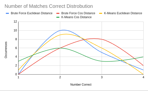
This chart shows how many times each number of matches was accomplished for each strategy. Here we can again see that although K-Means Cos Distance had the best peak performance, it also had nearly double the number of completely wrong category returns compared to the next highest (K-Means Euclidean Distance).

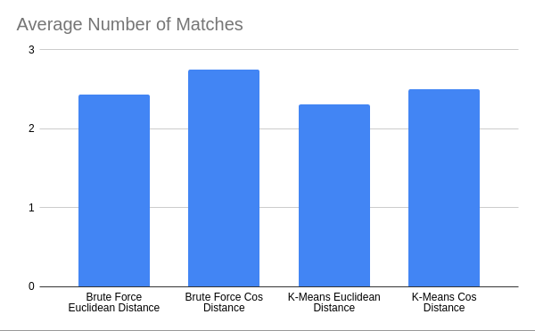
Finally, we also calculated the average number of connections achieved by each strategy. We don’t think this is particularly insightful.

Gephi

We wanted to visualize the connections between words that the word embedding imply, so we decided to dump an adjacency matrix for each connections game into gephi.

Gephi takes data like this in a simple CSV table like this one, where the values in the cells represent the strength of connection between words.

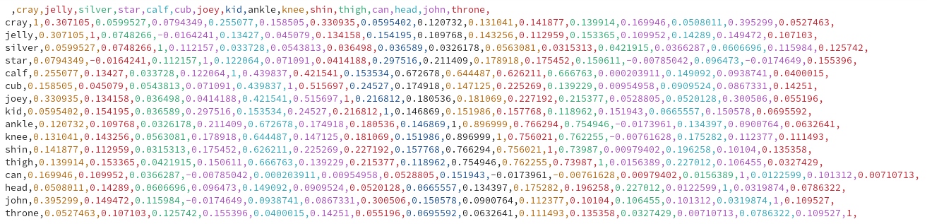
Really, this should be an upper or lower triangular matrix, because this adjacency matrix is symmetric. Fortunately, all values are relative to one another, so the duplicate reversed connection won’t really impact anything inside of Gephi.

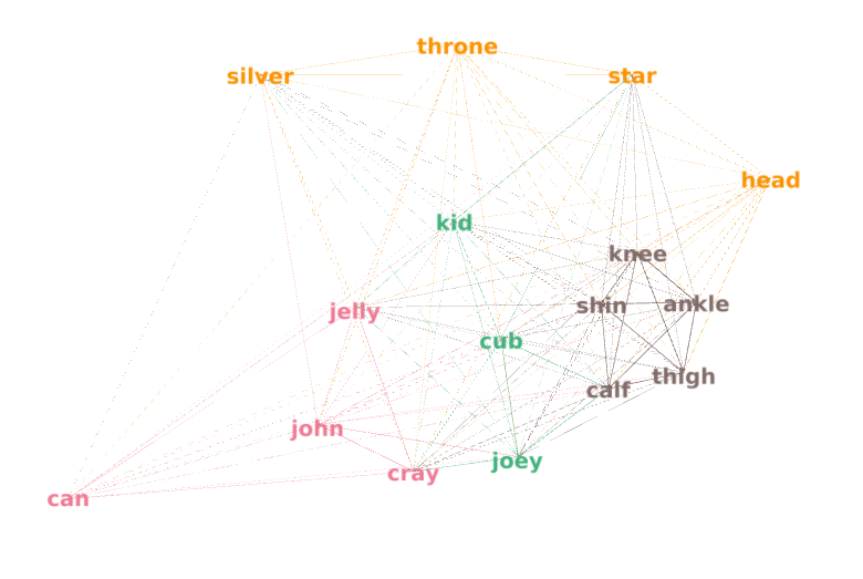
Inside of gephi, we simply set the layout algorithm to “ForceAtlas”, which iteratively produces a stable local equilibrium where all nodes repel one another equally and nodes’ attraction is set by the weight of edges connecting them.

More interestingly, we ran the “Modularity” calculation and adjusted the “resolution” parameter to achieve 4 clusters, which we set to be the colors of the nodes.

Modularity and Louvian Clustering explained soon!

This is the resulting graph for connections #7. We chose to analyze this game because it was most successfully solved by our program. You can see that a “leg parts” cluster is generated, but includes calf — meaning that calf is more often used in similar sentences to the other words in it’s assigned cluster than it is used in sentences similar to ones including kid, cub, and joey (young animals). It is however pulled close to it’s correct category by the layout algorithm. From here, it all falls apart. The other two categories are “words for restroom” and “words ending in fish”. Word anatomy isn’t captured in any way by CBOW embedding, and it doesn’t impact how words are used in similar sentences, so this makes sense.

Modularity

• aka, how easily can a network be divided into communities?
  It’s based on the density of internal connections vs external connections. Networks with high modularity have dense connections between nodes within modules and sparse connections between nodes in different modules
  
  (I didn’t draw the lines but you can imagine there being more within each community and a few branching out)

Here’s a fancy technical explanation:
“Modularity is defined as the difference between the number of edges within communities and the expected number of edges* in a random network with the same degree distribution.”

$$Q=\frac{1}{2m}\sum _{ij}\left(A_{ij}-\gamma \frac{k_i{k}_j}{2m}\right)\delta (ci,cj)$$

• $Q$ is the modularity
• $m$ is the total number of edges (or sum of the edge weights),
• $A_{ij}$ is the adjacency matrix (1 if there is an edge between nodes $i$ and $j$, 0 otherwise),
• $k_i$ and $k_j$ are the degrees of nodes $i$ and $j$,
• $\gamma$ is the resolution parameter (usually set to 1),
• $\delta (c_i,c_j)$ is 1 if nodes ii and jj are in the same community, 0 otherwise

* Expected number of edges: $\frac{n(n-1)p}{2}$ where $n$ is the nodes and $p$ is the probability of any two nodes being connected by an edge

Louvain algorithm

• a method designed to optimize the modularity of a graph - meaning creating denser internal communities and
  Two phase process:

1. Moving Nodes Locally: Each node is considered for potential reassignment to a different community based on the gain in modularity. Nodes are moved to the community that offers the highest increase in modularity.
2. Aggregation of the Network: After the local moving phase, communities are aggregated into super-nodes, forming a new network. This process is repeated until no further improvement in modularity can be achieved.
   The algorithm is also hierarchical, meaning it can recursively merge communities into larger groups (detection at multiple scales).
   

• The Louvain algorithm can also show disconnected communities or communities that are connected, but only in a very weak sense. Louvain may find arbitrarily badly connected communities.
• Time: Generally considered to be $O(N\log N)$ for $N$ nodes, though it can be approximated as $O(E)$ where $E$ is the number of edges (because the most time intensive operation involves calculating edge weights).

There’s a few variants to do things like handle weighted graphs, or the Leiden Algorithm that improves efficiency by only revisiting nodes whose neighborhoods have changed.

Next Steps / Things to try

• Modified k-means iteration to produce even size clusters
• Brute force sorting for minimum maximum distance from centroid (Think, circumscribed many dimensional sphere instead of average distance as it is now)
• More clustering algorithms in our program!!
• More algorithms and analysis in Gephi